Evaluation Study

Graph self-supervised learning (SSL) methods are compared by the accuracy of a linear classifier fitted on frozen node embeddings, on the assumption that a difference in that number comes from the pretraining objective. GraphSSL is the instrument of a controlled study of that assumption: how much of a reported result is the objective, and how much is the encoder it was trained with, the classifier that scores it, the data split, the seed and the training settings? A paper is in preparation; this page summarizes the design and the findings.

Design

• Eight objectives from six families: mutual information (DGI), contrastive learning with negatives (GraphCL, which at the node level coincides with GRACE), bootstrapping without negatives (BGRL, AFGRL), redundancy reduction (VICReg, Barlow Twins), self-distillation (GraphDINO) and masked feature reconstruction (GraphMAE).
• Three backbones: a 2-layer GCN, GIN and graph Transformer (256 units, batch norm).
• Six datasets: Cora, CiteSeer and PubMed (public split), Amazon Computers, Amazon Photo and Coauthor CS (a random 10/10/80 split as the standard one); and ogbn-arxiv, trained with neighbor sampling, also scored on its publication-year labels (arxiv-year), which neighbors rarely share.
• One shared, untuned protocol: 300 full-batch steps, AdamW (lr 5e-4), edge dropping and feature masking, 10 seeds (3 on ogbn-arxiv). It compares objectives at equal budget; the experiments below measure what that choice costs.
• Train once, evaluate many ways. Every model is saved. SSL training never sees a label, so the same embeddings are scored again with the linear probes of four public codebases (100 or 5,000 Adam steps, liblinear, and LogRegEvaluator, which standardizes the embeddings and chooses its L2 penalty on validation), with kNN, and on ten random splits.
• Two references for every number: the same encoder left untrained (same architecture and seed, scored identically), and logistic regression on the raw features. The first step (raw → untrained) is what the architecture adds; the second (untrained → trained) is what the objective adds.

Experiment	What varies	Levels
E1	objective × backbone	8 objectives, untrained encoder, 2 supervised references; 3 backbones; 6 datasets and ogbn-arxiv
E2	probe × split × labels	4 published linear probes, 3 controls, kNN; standard and 10 random splits; arxiv-year
E3	optimizer × learning rate	AdamW and SGD, 5 learning rates each; every backbone on Cora and CiteSeer, GCN on the Amazon and Coauthor graphs
E4	training step	14 evaluations between step 0 and 300, in three optimizer cells (Cora, CiteSeer)
E5	training budget	300 against 3,000 steps (GCN on Cora and the Amazon and Coauthor graphs; GIN and Transformer on Cora)
M	—	label-free metrics of every saved model: CKA between models, effective rank, uniformity, smoothing

Four analyses had their decision rules committed before their data existed: the label-free prediction test, the definitions summarizing the trajectories of E4, and the rules of E3 and E5 on the Amazon and Coauthor graphs.

A representation is mostly its backbone

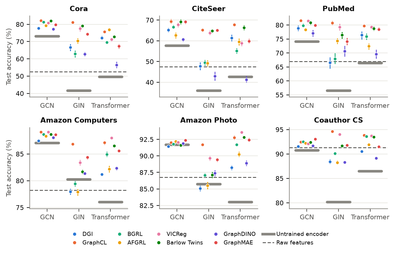
• An untrained GCN is already a good feature map on these graphs: 20.5, 10.2 and 7.1 points above the raw features on Cora, CiteSeer and PubMed. An untrained GIN or Transformer is not.
• The objectives repair weak feature maps more than they improve good ones. With a GCN the average objective adds 6.9, 8.6 and 5.6 points on the citation graphs but only 1.4, 0.2 and 1.5 on Amazon Computers, Amazon Photo and Coauthor CS; with a GIN, which starts 6 to 31 points lower, it adds 1.4 to 30.1.
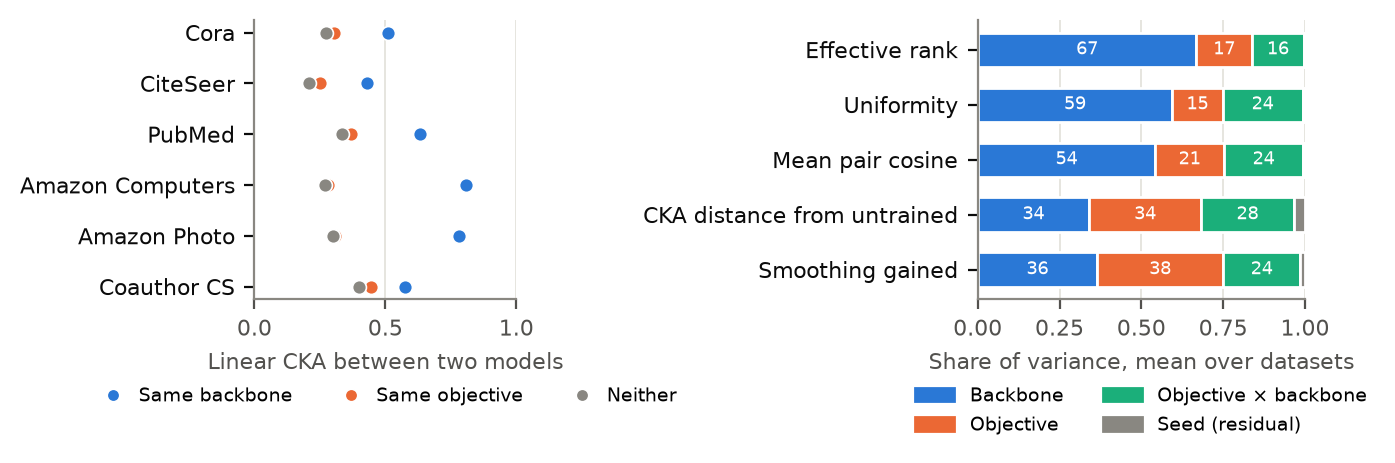
• Models resemble their backbone, not their objective. Two models that share a backbone have a linear CKA of 0.43 to 0.81, two that share an objective 0.25 to 0.45, barely above two that share neither. It holds across random initializations, and the masked autoencoder is no exception. With ten times the training budget the grouping weakens below the margin fixed in advance: it is a property of the shared budget.
• The backbone explains most of the gain: 68 to 82% of the variance of the gain over the untrained encoder on four of the six datasets.

The probe decides how large the gain looks

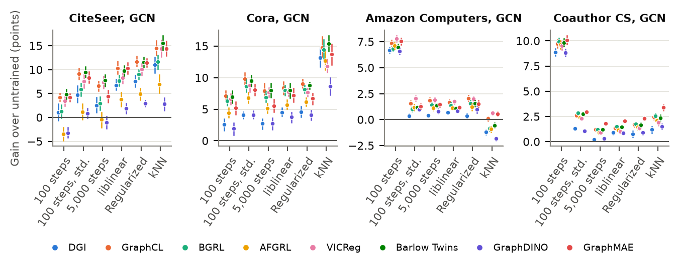
• In both directions. With a GCN, the 100-step probe of DGI and PyG-SSL measures an average gain of 1.5 points on CiteSeer, where the regularized probe measures 8.6, and 9.5 on Coauthor CS, where it measures 1.5. On ogbn-arxiv it finds gains of up to 22 points for GCN objectives that the regularized probe places at most 0.3 points above the untrained encoder.
• Two biases. An unregularized probe overfits trained embeddings when labels are few, which deflates the gain; and it underfits the untrained encoder, whose raw embeddings are 5 to 290 times smaller with a GCN, which inflates it. Which one wins depends on the number of labels.
• The fix is two settings: standardize the embeddings with the statistics of the training rows, and choose the L2 penalty on the validation split. LogRegEvaluator does both; liblinear with its penalty chosen on validation agrees with it.

What survives: the order within one backbone

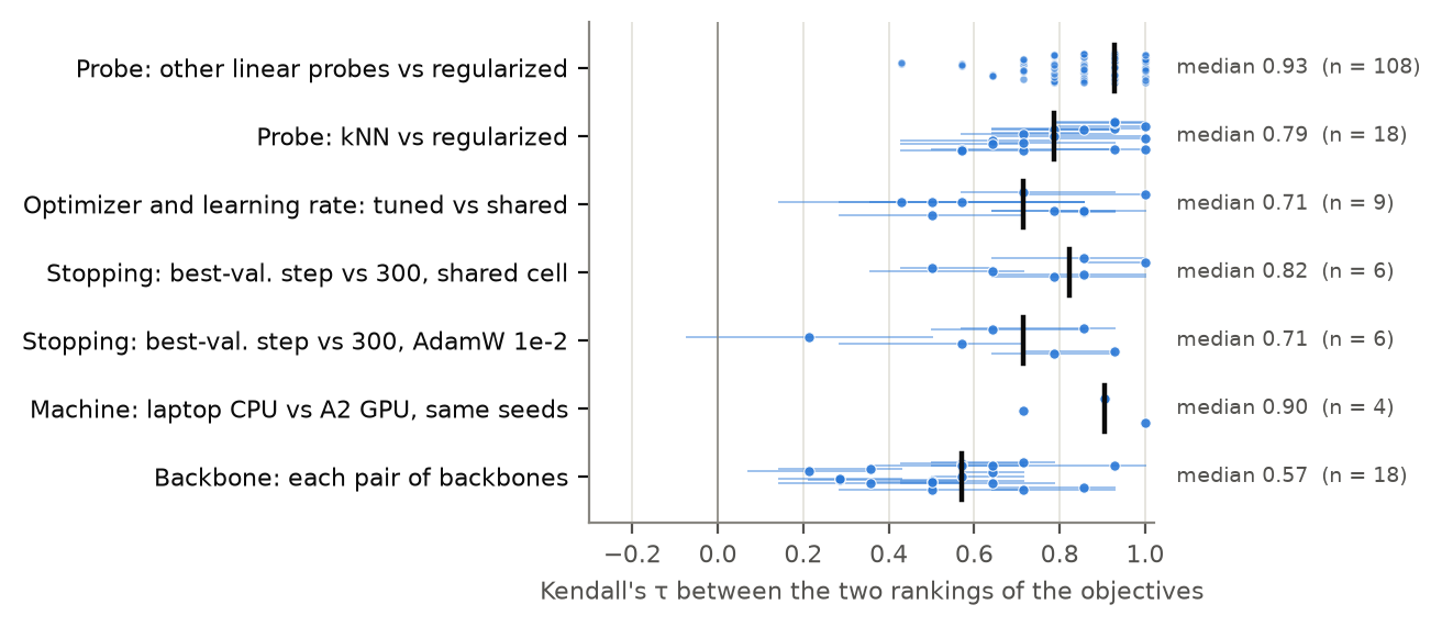
• The ranking of the objectives under one backbone holds across probes (median Kendall τ 0.93 over the linear probes) and machines, and partly across learning rates and stopping steps (τ 0.43 to 1.00), where GraphMAE, which peaks early and prefers a low learning rate, moves most.
• It does not hold across backbones: τ falls to 0.21 between two backbones, and on ogbn-arxiv the rankings of the GIN and the Transformer are reversed (τ = −0.79). A ranking of graph SSL objectives is a ranking for one backbone.
• GraphCL is the best objective in 13 of the 18 dataset–backbone cells.

The small gains hold against tuning and budget

The small GCN gains on the Amazon and Coauthor graphs are the result most exposed to "the protocol is untuned". Two tests with rules fixed before their runs asked whether tuning the optimizer and learning rate (E3), or ten times the training budget (E5), raises the average gain by a point or more on any of the three graphs. Neither does: the mean change is at most 0.2 points with tuning and 0.4 with the longer budget. Where gains are large, tuning helps: on Cora and CiteSeer it lifts the average objective by 1.0 to 7.6 points.

A larger graph, and labels that do not follow the edges

• On ogbn-arxiv, with a GCN, no objective improves on the untrained encoder under the regularized probe (from 5.6 points below to 0.3 above), although a supervised GCN reaches 71.74% in the OGB benchmark, about 2.5 points more. With a GIN seven of eight objectives gain, by up to 8.4 points; with the Transformer only AFGRL does. The probe is the largest factor of the gain on this graph.
• On the year labels every GCN objective gains 2.0 to 2.6 points, while every GIN objective loses: the effect belongs to the backbone as much as to the objectives.

Label-free metrics barely tell which objective helped

A test fixed in advance asked whether a metric computed without labels (effective rank, CKA distance from the untrained encoder, neighbor smoothing gained, uniformity) picks the objective that gains most. Only the CKA distance passes, and narrowly: the objective it ranks first loses 2.90 points against the best one, a random choice 2.99, and leaving ogbn-arxiv or Amazon Photo out of the test set reverses the verdict. Effective rank points the wrong way: across objectives on one backbone, a higher rank goes with a smaller gain.

A seed does not pin a result down

The GCN and GIN models of Cora and CiteSeer were trained twice with the same seeds and configuration, on a GPU server and on a laptop CPU. Models are initialized on the CPU, so the initial weights match; the augmentations draw from the generator of the device that holds the graph, so they do not. With a GCN a seed differs from its rerun by about half of what two independent seeds differ by, with a GIN by about three quarters; the means over ten seeds and the order of the objectives survive (τ 0.71 to 1.00). Compare means over seeds, never one seed against the same seed on another machine.

How much of the result is the method?

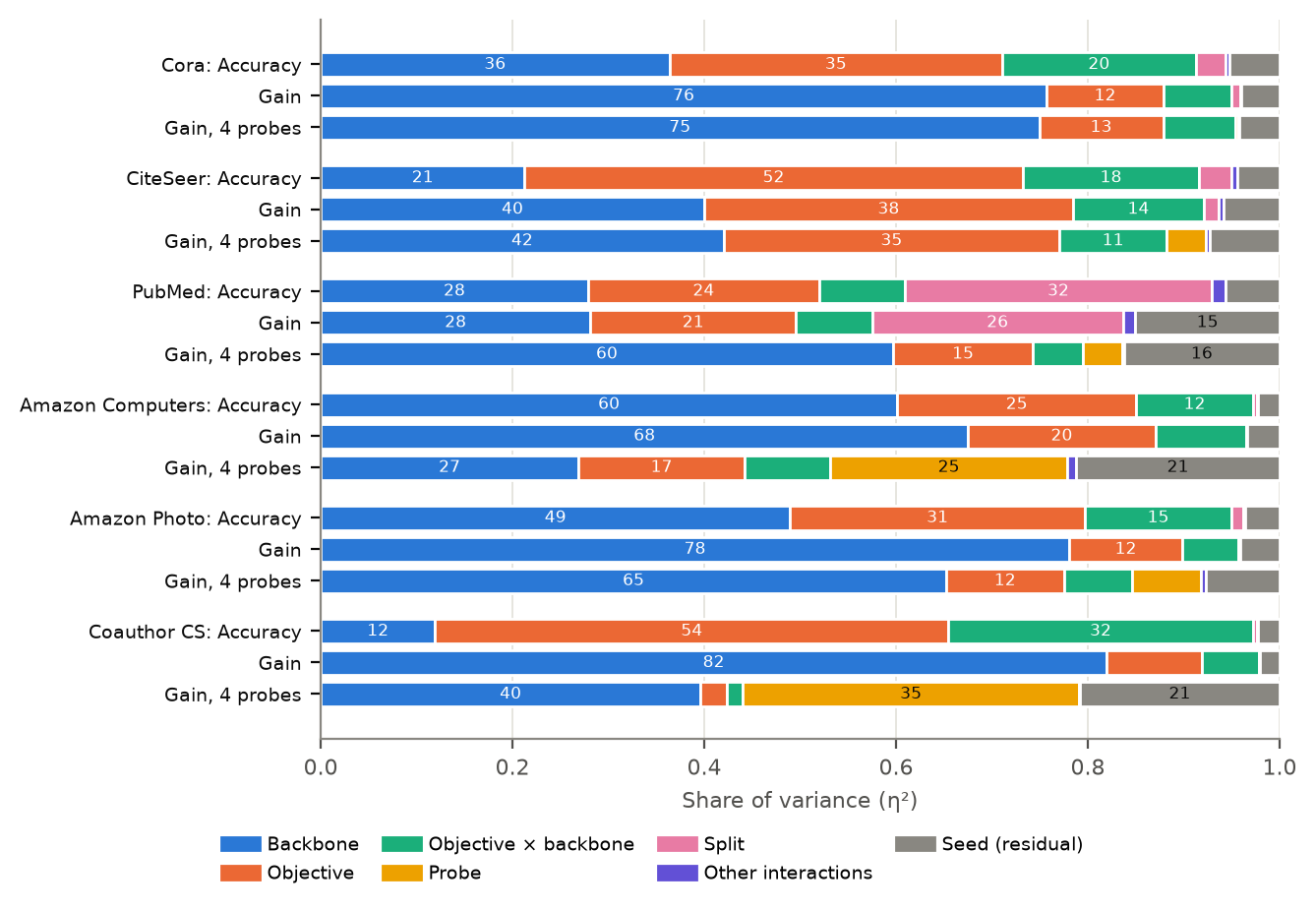
On these graphs and with this protocol, the objective explains between a quarter and a half of the variation of a reported accuracy, part of which depends on the backbone it is paired with, and much less of what SSL adds over the encoder it started from. The shares describe this grid of experiments; they are not causal estimates.

Recommendations

1. Report the untrained encoder and the raw features, scored in the same way, and the gain over the untrained encoder.
2. Regularize the probe on validation data: standardize the embeddings and choose the L2 penalty on the validation split. Report the solver, the grid and whether the fit converged.
3. Select nothing on the test split, neither the pretraining epoch nor a probe setting.
4. Use more than one backbone, or say why one is enough, and report the ranking under each.
5. Use ten seeds or more, report intervals, and compare means over seeds, not seeds across machines.
6. Report the trajectory, or at least whether accuracy declines after its best validation step.
7. Do not choose an objective by effective rank.

What this does not show

• One untuned configuration per objective, and tuning beyond the optimizer and learning rate (augmentations, width, depth) is not studied.
• Node classification only, transductive, on graphs where neighbors tend to share labels, except for the year labels of ogbn-arxiv.
• The probes of other codebases are re-implementations applied to GraphSSL's embeddings, not runs of those codebases' own pipelines.
• The device is fixed within a dataset and experiment but differs between datasets.

Reproduce

Every number comes from the result files in benchmarks/paper/: one JSON per run with per-seed metrics, the exact model configuration, the git commit and the package versions. Training is driven by benchmarks/paper_runs.sh (Cora and CiteSeer) and benchmarks/paper_v2.sh (the other datasets, ogbn-arxiv, E3, probes and metrics; see their headers), and the analysis by:

P=benchmarks/paper
python benchmarks/analyze_factors.py $P/probes/*/probes__*.json --untrained-root $P/models_untrained --out $P/analysis
python benchmarks/analyze_representations.py --metrics $P/metrics/*/metrics__*.json \
  --probes $P/probes/*/probes__*.json --untrained-root $P/models_untrained --out $P/analysis
python benchmarks/analyze_e3.py           # E3: shared vs tuned, the decision rule
python benchmarks/analyze_trajectories.py # E4
python benchmarks/analyze_e5.py           # E5: training budget, the decision rule
python benchmarks/paper_figures_v2.py     # the figures on this page

The summaries of E3, E4 and E5, with every per-objective number, are in benchmarks/paper/analysis/{e3,trajectories,e5}/summary.md. Trained models are not committed.